Types of Optimization algorithms and Optimizing Gradient Descent

Have you ever wondered which optimization algorithm to use for your Neural network Model to produce slightly better and faster results by updating the Model parameters such as Weights and Bias values? Should we use Gradient Descent or Stochastic gradient Descent or Adam?

I too didn’t know about the major differences between these different types of Optimization Strategies and which one is better over another before writing this article.

NOTE: Having a good theoretical knowledge is amazing but implementing them in code in a real-time deep learning project is a completely different thing. You might get different and unexpected results based on different problems and datasets. So as a Bonus,I am also adding the links to the various courses which has helped me a lot in my journey to learn Data science and ML, experiment and compare different optimization strategies which led me to write this article on comparisons between different optimizers while implementing deep learning and comparing the different optimization strategies. Below are some of the resources which have helped me a lot to become what I am today. I am personally a fan of DataCamp, I started from it and I am still learning through DataCamp and keep doing new courses. They seriously have some exciting courses. Do check them out.

Also, I have noticed that DataCamp is having a SALE(75%off) on all the courses. So this would literally be the best time to grab some yearly subscriptions(which I have) which basically has unlimited access to all the courses and other things on DataCamp and make fruitful use of your time sitting at home during this Pandemic.So go for it folks and Happy learning, make the best use of this quarantine time and come out of this pandemic stronger and more skilled.

1)This is the link to the course by DataCamp on Deep learning in python using Keras package or definitely you can start with Building CNN for image processing using keras . If understanding deep learning and AI fundamentals is what you want right now then the above 2 courses are the best deep learning courses you can find out there to learn fundamentals of deep learning and also implement it in python. These were my first Deep learning course which has helped me a lot to properly understand the basics.

2)These courses on Building chatbots in Python and NLP fundamentals in Python using NLTK are also recommended for people interested more in learning AI and deep learning. So go give it a try on the basis of your interest.

3) Machine learning in Python using Scikit-learn- This course will teach you how to implement supervised learning algorithms in python with different datasets.

4)Data wrangling and manipulating Data Frames using Pandas-This amazing course will help you perform data wrangling and data pre-processing in python. And a data scientist spends most of his time doing pre-processing and data wrangling. So this course might come out to be handy for beginners.

5) This course teaches you the Intermediate level Python for Data science and this foundation course on Data scientist with python is the best option if you want to start you career as a data scientist and learn all the required fundamentals in the industry today using Python.

6) Recently Data camp has started an new program where they are providing various real world Projects and problems statements to help data enthusiasts build a strong practical data science foundation along with their courses. So try any of these Projects out. It is surely very exciting and will help you learn faster and better. Recently I completed a project on Exploring the evolution of Linux and it was an amazing experience.

7) R users , don’t worry I also have some hand picked best R courses for you to get started with building data science and Machine learning foundations and also doing it side by side using this amazing Data science with R course which will teach you the complete fundamentals. Trust me this one is worth your time and energy.

8) This course is also one of the best for understanding basics of Machine learning in R called Machine learning Toolbox .

9) All data science projects start from exploring the data and it is one of the most important tasks for a data scientist to know the dataset inside out so this lovely course on Exploratory data analysis using R is what you need to start any data analytics and data science project. Also this course on Statistical modelling in R would be useful for all the aspiring data scientists like me.Statistics is the foundation of data science.

10) Pre-processing data for machine learning tasks is another handy course for deep learning and ML enthusiasts, as it is one of the most important and first tasks you perform for any data science project.

P.S: I am still using DataCamp and keep doing courses in my free time. I actually insist the readers to try out any of the above courses as per their interest, to get started and build a good foundation in Machine learning and Data Science. The best thing about these courses by DataCamp is that they explain it in a very elegant and different manner with a balanced focus on practical and well as conceptual knowledge and at the end, there is always a Case study. This is what I love the most about them. These courses are truly worth your time and money. These courses would surely help you also understand and implement Deep learning, machine learning in a better way and also implement it in Python or R. I am damn sure you will love it and I am claiming this from my personal opinion and experience.

Coming back to the topic-

What are Optimization Algorithms?

Optimization algorithms help us to minimize (or maximize) an Objective function (another name for Error function) E(x) which is simply a mathematical function dependent on the Model’s internal learnable parameters which are used in computing the target values(Y) from the set of predictors(X) used in the model. For example — we call the Weights(W) and the Bias(b) values of the neural network as its internal learnable parameters which are used in computing the output values and are learned and updated in the direction of optimal solution i.e minimizing the Loss by the network’s training process and also play a major role in the training process of the Neural Network Model. The internal parameters of a Model play a very important role in efficiently and effectively training a Model and produce accurate results. This is why we use various Optimization strategies and algorithms to update and calculate appropriate and optimum values of such a model’s parameters which influence our Model’s learning process and the output of a Model.

Types of optimization algorithms?

Optimization Algorithm falls in 2 major categories :

First Order Optimization Algorithms — These algorithms minimize or maximize a Loss function E(x) using its Gradient values with respect to the parameters. Most widely used First-order optimization algorithm is Gradient Descent. The First order derivative tells us whether the function is decreasing or increasing at a particular point. First-order Derivative basically give us a line which is tangential to a point on its Error Surface. What is the Gradient of a function?

A Gradient is simply a vector which is a multi-variable generalization of a derivative(dy/dx) which is the instantaneous rate of change of y with respect to x. The difference is that to calculate a derivative of a function which is dependent on more than one variable or multiple variables, a Gradient takes its place. And a gradient is calculated using Partial Derivatives. Also, another major difference between the Gradient and a derivative is that a Gradient of a function produces a Vector Field.

A Gradient is represented by a Jacobian Matrix — which is simply a Matrix consisting of first-order partial Derivatives(Gradients).

Hence summing up, a derivative is simply defined for a function dependent on single variables , whereas a Gradient is defined for function dependent on multiple variables. Now let’s not get more into Calculas and Physics.

2. Second-Order Optimization Algorithms — Second-order methods use the second-order derivative which is also called Hessian to minimize or maximize the Loss function. The Hessian is a Matrix of Second Order Partial Derivatives. Since the second derivative is costly to compute, the second-order is not used much. The second-order derivative tells us whether the first derivative is increasing or decreasing which hints at the function’s curvature. Second-Order Derivative provide us with a quadratic surface which touches the curvature of the Error Surface.

Some Advantages of Second-Order Optimization over First Order —

Although the Second Order Derivative may be a bit costly to find and calculate, the advantage of a Second-order Optimization Technique is that does not neglect or ignore the curvature of Surface. Secondly, in terms of Step-wise Performance, they are better.

You can search more on second-order Optimization Algorithms here-https://web.stanford.edu/class/msande311/lecture13.pdf

So which Order Optimization Strategy to use?

Now, The First Order Optimization techniques are easy to compute and less time consuming, converging pretty fast on large data sets.

Second-Order Techniques are faster only when the Second Order Derivative is known otherwise, these methods are always slower and costly to compute in terms of both time and memory.

Although ,sometimes Newton’s Second Order Optimization technique can sometimes Outperform First Order Gradient Descent Techniques because Second Order Techniques will not get stuck around paths of slow convergence around saddle points whereas Gradient Descent sometimes gets stuck and does not converges.

Best way to know which one converges fast is to try it out yourself.

Now, what are the different types of Optimization Algorithms used in Neural Networks?

Gradient Descent

Gradient Descent is the most important technique and the foundation of how we train and optimize Intelligent Systems. What is does is —

“Oh Gradient Descent — Find the Minima , control the variance and then update the Model’s parameters and finally lead us to Convergence”

θ=θ−η⋅∇J(θ) — is the formula of the parameter updates, where ‘η’ is the learning rate,’∇J(θ)’ is the Gradient of Loss function-J(θ) w.r.t parameters-‘θ’.

It is the most popular Optimization algorithms used in optimizing a Neural Network. Now gradient descent is majorly used to do Weights updates in a Neural Network Model, i.e update and tune the Model’s parameters in a direction so that we can minimize the Loss function. Now we all know a Neural Network trains via a famous technique called Backpropagation, in which we first propagate forward calculating the dot product of Inputs signals and their corresponding Weights and then apply an activation function to those sum of products, which transforms the input signal to an output signal and also is important to model complex Non-linear functions and introduces Non-linearities to the Model which enables the Model to learn almost any arbitrary functional mappings.

After this, we propagate backwards in the Network carrying Error terms and updating Weights values using Gradient Descent, in which we calculate the gradient of Error(E) function with respect to the Weights (W) or the parameters, and update the parameters (here Weights) in the opposite direction of the Gradient of the Loss function w.r.t to the Model’s parameters.

Weight updates in the opposite direction of the Gradient

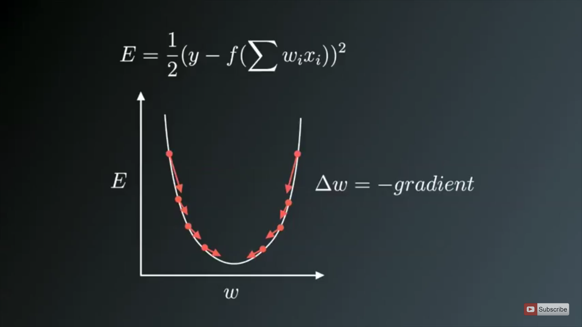
The image on above shows the process of Weight updates in the opposite direction of the Gradient Vector of Error w.r.t to the Weights of the Network. The U-Shaped curve is the Gradient(slope). As one can notice if the Weight(W) values are too small or too large then we have large Errors , so want to update and optimize the weights such that it is neither too small nor too large , so we descent downwards opposite to the Gradients until we find a local minima.

Variants of Gradient Descent-

The traditional Batch Gradient Descent will calculate the gradient of the whole Data set but will perform only one update, hence it can be very slow and hard to control for datasets which are very very large and don’t fit in the Memory. How big or small of an update to do is determined by the Learning Rate -η, and it is guaranteed to converge to the global minimum for convex error surfaces and to a local minimum for non-convex surfaces. Another thing while using Standard batch Gradient descent is that it computes redundant updates for large data sets.

The above problems of Standard Gradient Descent are rectified in Stochastic Gradient Descent.

1. Stochastic gradient descent

Stochastic Gradient Descent(SGD) on the other hand performs a parameter update for each training example. It is usually a much faster technique. It performs one update at a time.

θ=θ−η⋅∇J(θ;x(i);y(i)) , where {x(i) ,y(i)} are the training examples.

Now due to these frequent updates, parameters updates have high variance and causes the Loss function to fluctuate to different intensities. This is actually a good thing because it helps us discover new and possibly better local minima, whereas Standard Gradient Descent will only converge to the minimum of the basin as mentioned above.

But the problem with SGD is that due to the frequent updates and fluctuations it ultimately complicates the convergence to the exact minimum and will keep overshooting due to the frequent fluctuations.

Although, it has been shown that as we slowly decrease the learning rate-η, SGD shows the same convergence pattern as Standard gradient descent.

High Variance parameter updates for each training example cause the Loss function to fluctuate heavily due to which we might not get the minimum value of the parameter which gives us the least Loss value.

The problems of high variance parameter updates and unstable convergence can be rectified in another variant called mini-batch Gradient Descent.

2. Mini Batch Gradient Descent

An improvement to avoid all the problems and demerits of SGD and standard Gradient Descent would be to use Mini Batch Gradient Descent as it takes the best of both techniques and performs an update for every batch with n training examples in each batch.

The advantages of using Mini Batch Gradient Descent are —

It Reduces the variance in the parameter updates, which can ultimately lead us to much better and stable convergence.

Can make use of highly optimized matrix optimizations common to state-of-the-art deep learning libraries that make computing the gradient w.r.t. a mini-batch very efficient.

Commonly Mini-batch sizes Range from 50 to 256 but can vary as per the application and problem being solved.

Mini-batch gradient descent is typically the algorithm of choice when training a neural network nowadays

P.S —Actually the term SGD is used also when mini-batch gradient descent is used.

Challenges faced while using Gradient Descent and its variants —

Choosing a proper learning rate can be difficult. A learning rate that is too small leads to painfully slow convergence i.e will result in small baby steps towards finding optimal parameter values which minimize loss and finding that valley which directly affects the overall training time which gets too large. While a learning rate that is too large can hinder convergence and cause the loss function to fluctuate around the minimum or even to diverge.

Additionally, the same learning rate applies to all parameter updates. If our data is sparse and our features have very different frequencies, we might not want to update all of them to the same extent, but perform a larger update for rarely occurring features.

Another key challenge of minimizing highly non-convex error functions common for neural networks is avoiding getting trapped in their numerous sub-optimal local minima. Actually, Difficulty arises in fact not from local minima but from saddle points, i.e. points where one dimension slopes up and another slope down. These saddle points are usually surrounded by a plateau of the same error, which makes it notoriously hard for SGD to escape, as the gradient is close to zero in all dimensions.

Optimizing the Gradient Descent

Now we will discuss the various algorithms which are used to further optimize Gradient Descent.

Momentum

V(t)=γV(t−1)+η∇J(θ).

and finally, we update parameters by θ=θ−V(t).

The momentum term γ is usually set to 0.9 or similar value.

Here the momentum is the same as the momentum in classical physics, as we throw a ball down a hill it gathers momentum and its velocity keeps on increasing.

The same thing happens with our parameter updates —

It leads to faster and stable convergence.

Reduced Oscillations

The momentum term γ increases for dimensions whose gradients point in the same directions and reduces updates for dimensions whose gradients change directions. This means it does parameter updates only for relevant examples. This reduces the unnecessary parameter updates which lead to faster and stable convergence and reduced oscillations.

Nesterov accelerated gradient

A researcher named Yurii Nesterov saw a problem with Momentum —

However, a ball that rolls down a hill, blindly following the slope, is highly unsatisfactory. We’d like to have a smarter ball, a ball that has a notion of where it is going so that it knows to slow down before the hill slopes up again.

What actually happens is that as we reach the minima i.e the lowest point on the curve, the momentum is pretty high and it doesn’t know to slow down at that point due to the high momentum which could cause it to miss the minima entirely and continue movie up. This problem was noticed by Yurii Nesterov.

He published a research paper in 1983 which solved this problem of momentum and we now call this strategy Nesterov Accelerated Gradient.

In the method, he suggested we first make a big jump based on the previous momentum then calculate the Gradient and them make a correction which results in a parameter update. Now, this anticipatory update prevents us to go too fast and not miss the minima and makes it more responsive to changes.

Nesterov accelerated gradient (NAG) is a way to give our momentum term this kind of prescience. We know that we will use our momentum term γV(t−1) to move the parameters θ. Computing (θ−γV(t−1)) thus gives us an approximation of the next position of the parameters which gives us a rough idea where our parameters are going to be. We can now effectively look ahead by calculating the gradient not w.r.t. to our current parameters θ but w.r.t. the approximate future position of our parameters:

V(t)=γV(t−1)+η∇J( θ−γV(t−1) ) and then update the parameters using θ=θ−V(t).

One can refer more on NAGs here http://cs231n.github.io/neural-networks-3/.

Now that we are able to adapt our updates to the slope of our error function and speed up SGD in turn, we would also like to adapt our updates to each individual parameter to perform larger or smaller updates depending on their importance.

Adagrad

It simply allows the learning Rate -η to adapt based on the parameters. So it makes big updates for infrequent parameters and small updates for frequent parameters. For this reason, it is well-suited for dealing with sparse data.

It uses a different learning Rate for every parameter θ at a time step based on the past gradients which were computed for that parameter.

Previously, we performed an update for all parameters θ at once as every parameter θ(i) used the same learning rate η. As Adagrad uses a different learning rate for every parameter θ(i) at every time step t, we first show Adagrad’s per-parameter update, which we then vectorize. For brevity, we set g(t,i) to be the gradient of the loss function w.r.t. to the parameter θ(i) at time step t.

Adagrad modifies the general learning rate η at each time step t for every parameter θ(i) based on the past gradients that have been computed for θ(i).

The main benefit of Adagrad is that we don’t need to manually tune the learning rate. Most implementations use a default value of 0.01 and leave it at that.

Disadvantage —

Its main weakness is that its learning rate-η is always Decreasing and decaying.

This happens due to the accumulation of each squared Gradients in the denominator since every added term is positive. The accumulated sum keeps growing during training. This, in turn, causes the learning rate to shrink and eventually become so small, that the model just stops learning entirely and stops acquiring new additional knowledge. Because we know that as the learning rate gets smaller and smaller the ability of the Model to learn fastly decreases and which gives very slow convergence and takes very long to train and learn i.e learning speed suffers and decreases.

This problem of Decaying learning Rate is Rectified in another algorithm called AdaDelta.

AdaDelta

It is an extension of AdaGrad which tends to remove the decaying learning Rate problem of it. Instead of accumulating all previously squared gradients, Adadelta limits the window of accumulated past gradients to some fixed size w.

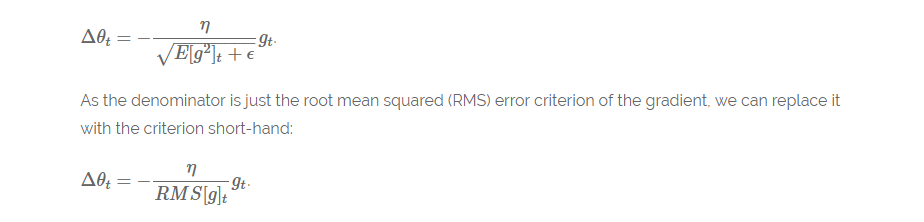
Instead of inefficiently storing w previous squared gradients, the sum of gradients is recursively defined as a decaying mean of all past squared gradients. The running average E[g²](t) at time step t then depends (as a fraction γ similarly to the Momentum term) only on the previous average and the current gradient.

E[g²](t)=γ.E[g²](t−1)+(1−γ).g²(t) , We set γ to a similar value as the momentum term, around 0.9.

Δθ(t)=−η⋅g(t,i).

θ(t+1)=θ(t)+Δθ(t).

Another thing with AdaDelta is that we don’t even need to set a default learning Rate.

What Improvements we have done so far —

We are calculating different learning Rates for each parameter.

We are also calculating momentum.

Preventing Vanishing(decaying) learning Rates.

What more improvements can we do?

Since we are calculating individual learning rates for each parameter , why not calculate individual momentum changes for each parameter and store them separately. This is where a new modified technique and improvement comes into play called as Adam.

Adam

Adam stands for Adaptive Moment Estimation. Adaptive Moment Estimation (Adam) is another method that computes adaptive learning rates for each parameter. In addition to storing an exponentially decaying average of past squared gradients like AdaDelta, Adam also keeps an exponentially decaying average of past gradients M(t), similar to momentum:

M(t) and V(t) are values of the first moment which is the Mean and the second moment which is the uncentered variance of the gradients respectively.

The formulas for the first Moment(mean) and the second moment (the variance) of the Gradients

Then the final formula for the Parameter update is —

The values for β1 is 0.9 , 0.999 for β2, and (10 x exp(-8)) for ϵ.

Adam works well in practice and compares favourably to other adaptive learning-method algorithms as it converges very fast and the learning speed of the Model is quiet Fast and efficient and also it rectifies every problem that is faced in other optimization techniques such as vanishing Learning rate, slow convergence of High variance in the parameter updates which leads to fluctuating Loss function

Visualization of the Optimization Algorithms

SGD optimization on loss surface contours

From the above images, one can see that the Adaptive algorithms converge very fast and quickly find the right direction in which parameter updates should occur. Whereas standard SGD, NAG and momentum techniques are very slow and could not find the right direction.

Conclusion

Which optimizer should we use?

The question was to choose the best optimizer for our Neural Network Model in order to converge fast and to learn properly and tune the internal parameters so as to minimize the Loss function.

Adam works well in practice and outperforms other Adaptive techniques.

If your input data is sparse then methods such as SGD, NAG and momentum are inferior and perform poorly. For sparse data sets, one should use one of the adaptive learning-rate methods. An additional benefit is that we won’t need to adjust the learning rate but likely achieve the best results with the default value.

If one wants fast convergence and train a Deep Neural Network Model or a highly complex Neural Network then Adam or any other Adaptive learning rate techniques should be used because they outperform every other optimization algorithms.

I hope you guys liked the article and were able to give you a good intuition towards the different behaviours of different Optimization Algorithms.You can reach out to me on the following social profiles below for any doubts or queries and follow me there as well.

Stay safe and stay indoors and make sure to make the best use of your time during this lockdown.

References —

Optimizing Gradient Descent- http://sebastianruder.com/optimizing-gradient-descent/

Dean, J., Corrado, G. S., Monga, R., Chen, K., Devin, M., Le, Q. V, … Ng, A. Y. (2012). Large Scale Distributed Deep Networks. NIPS 2012: Neural Information Processing Systems. http://doi.org/10.1109/ICDAR.2011.95

Ioffe, S., & Szegedy, C. (2015). Batch Normalization : Accelerating Deep Network Training by Reducing Internal Covariate Shift. arXiv Preprint arXiv:1502.03167v3.

Qian, N. (1999). On the momentum term in gradient descent learning algorithms. Neural Networks : The Official Journal of the International Neural Network Society, 12(1), 145–151. http://doi.org/10.1016/S0893-6080(98)00116-6

Kingma, D. P., & Ba, J. L. (2015). Adam: a Method for Stochastic Optimization. International Conference on Learning Representations

Zaremba, W., & Sutskever, I. (2014). Learning to Execute, 1–25. Retrieved from http://arxiv.org/abs/1410.4615

Zhang, S., Choromanska, A., & LeCun, Y. (2015). Deep learning with Elastic Averaging SGD. Neural Information Processing Systems Conference (NIPS 2015).Retrieved from http://arxiv.org/abs/1412.6651

Darken, C., Chang, J., & Moody, J. (1992). Learning rate schedules for faster stochastic gradient search. Neural Networks for Signal Processing II Proceedings of the 1992 IEEE Workshop, (September). http://doi.org/10.1109/NNSP.1992.253713

MODULAR MACHINE LEARNING

Search This Blog